THE RESULT
What the data shows
Across 7,608 complete test hours, MAE is 0.451 kWh, only 1.2% below the selected baseline. The nominal 90% interval covers 87.9% of test hours.
The day-bootstrap interval for the MAE advantage crosses zero. These results do not establish that the more complex model is preferable to the simple baseline.
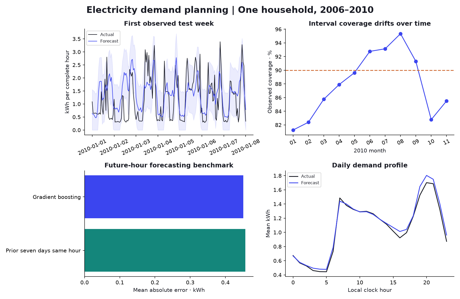
| model | test hours | mae kwh | rmse kwh |
|---|---|---|---|
| Prior seven days same hour | 7,608 | 0.4566 | 0.6426 |
| Gradient boosting | 7,608 | 0.451 | 0.6131 |
A complete analytical workflow
2,075,259 source observations, a reproducible SQL data mart, chronological experiments, an executed notebook, and an interactive dashboard.
Explore the results and assumptions ↗Data contract
One source row is a minute clock observation. An observed minute contributes Global_active_power / 60 kWh. Hourly energy is a valid target only if 60 readings exist; partial sums remain separately identified observed energy. The complete source calendar contains missing measurements. At midnight the model forecasts all hours of the coming day from finalized prior-day readings; no contemporaneous meter or weather measurement enters the predictors.
Model decisions
A fixed gradient-boosting regressor is compared to previous-day, previous-week and prior-seven-day same-hour baselines. January–June 2009 MAE selects the baseline and model size. July–December 2009 absolute residuals calibrate a nominal 90% interval with a finite-sample quantile; the lower bound is clipped at zero. January–November 2010 remains untouched for testing. All target hours need complete measurements. Coverage is empirical, not a guarantee. The bootstrap uses calendar-day clusters, not independent hours.
Read the operating runbook ↓THE METHOD
From source to answer
Minute-level energy accounting, SQL hourly aggregation, complete-hour target rules, day-ahead lag features, chronological baseline/model selection, separate residual calibration, temporal coverage diagnostics, and an editable tariff scenario.
- Ingest the original minute observations and record source provenance.
- Convert minute-average kW to kWh; accept hourly targets only with all 60 readings.
- Create features from prior days available before each forecast midnight.
- Train in 2007–2008, select in early 2009, calibrate in late 2009, and test in 2010.
- Report error, missing-hour coverage and interval coverage separately; expose tariff assumptions.
The Python source exposes this study’s transformations. The complete project download includes shared preparation and evaluation routines.
EVALUATION
How the result was checked
2007–2008 training; January–June 2009 configuration and baseline selection; July–December 2009 interval calibration; January–November 2010 untouched testing. Only hours with 60 observed minute readings are scored.
Select lowest validation MAE; freeze fit. Calibrate a nominal 90% symmetric residual band on a separate six-month block. Test dates are never used for selection.
Target and input features
Target: Energy in a complete clock hour, kWh
Inputs: hour, weekday, month, lag_24, lag_48, lag_168, lag_336, prior_week_same_hour
THE NEXT DECISION
What follows from the finding
Retain the simple baseline unless a new evaluation establishes a useful operational gain. Investigate missing readings and seasonal interval coverage before a monitored forecasting pilot. Use tariff scenarios only with explicitly supplied rates.
Where the conclusion stops
This is one historical household, not a utility fleet or current tariff study. Local timestamps lack DST/UTC disambiguation. Incomplete hours are unknown and excluded from scoring. Time dependence undermines exchangeability assumptions behind residual bands. The paired day bootstrap does not preserve dependence between adjacent days. Illustrative tariff comparisons are arithmetic scenarios and show no demand-shifting savings.
Related studies may reuse observations or holdouts. These are historical analyses; associations and backtests do not demonstrate commercial impact. Further model tuning needs new, untouched evaluation data.